Classifying Tweets with Keras and TensorFlow
Summer is drawing to a close. The air is humid and still. You’re between projects at work. What do you do with these few empty days?
If you’re like me, you train a neural net. It had been on my “To Do” list for about a year now, and while I had done some reading and tutorials, I hadn’t yet made my own from the ground up.
I spent a few days chasing dead-ish ends, doing even more tutorials, and tinkering. I emerged with a custom neural net that could classify text as positive or negative with 79.3% accuracy.
Here’s how to create your own neural net using Python, TensorFlow, and Keras! Happy learnings ✨
So what do neural nets do?
Neural net[work]s are collections of nodes that apply transformations to data. Their core behavior is: given an input, generate an output.
The intriguing aspect of neural nets is that we don’t tell them how to generate that output. Rather, we set them up to “learn” how to generate outputs based on massive amounts of training data. Training data consists of an input and an output, usually labelled by humans. The neural net intakes a piece of training data, generates an output, compares that output to the actual result, and adjusts the weights on its nodes — that is, how likely an individual node is to return a certain intermediate value. Modifying these weights leads a net to return one value or another given an input, and is how the net refines its accuracy as it trains.
A neural network with two hidden layers. Source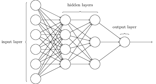
Nodes are arranged in layers within the neural net. All neural nets have an input layer and an output layer; within, they have at least one additional “hidden” layer. “Deep” neural nets have more than one hidden layer. This is also the difference, name-wise, between “machine” and “deep” learning. Once you train a neural net, it contains a fairly accurate self-adjusted system for creating outputs. Ideally, you can feed novel data into the net and end up with a meaningful output.
Neural nets can either classify extant data or predict new data. Identifying musical genre is an example of the former; fusing visual styles, of the latter. Kristen Stewart -- yes, the lead from Twilight -- used this to give her film Come Swim (2017) an impressionist look. She even co-authored a paper about the technique 🔥🔥🔥
Fine-tuning the visual treatment for Come Swim. Source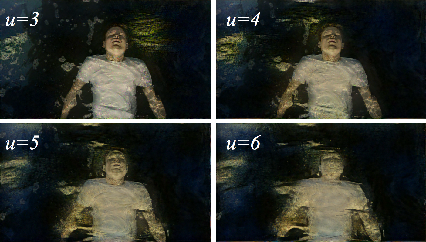
Deep Dream, a project out of Google, both classifies and predicts. It uses classifications to suggest predictions, which in turn amplify the certainty of classifications. It turns landscapes and portraits into fields of roiling curves often resembling human eyes.
A sample of what Deep Dream can do when applied to Edvard Munch's The Scream. Source
I won’t get into the specifics of neural nets or training/adjustment mechanics here. I’ve done some reading but I have a long way to go before I am truly 1337. I highly recommend Neural Networks and Deep Learning if you’re looking for a great intro to the field.
What’s our neural net going to do?
We’ll perform the relatively straightforward task of classifying text — specifically, we’ll predict whether text expresses a positive or a negative sentiment. As training data, we’re using the behemoth Twitter Sentiment Analysis Dataset documented at ThinkNook.
Getting started: environment and tools
Our neural net is Python 2 based, so make sure that’s what you’re working with on your own machine. I highly recommend virtualenv for managing your package installs, and IPython as an interactive editor. The net itself will be built using TensorFlow, an open-source, Google-backed machine learning framework. We’re laying Keras on top of TensorFlow to act as an API and simplify TensorFlow’s syntax. If you want to dig into TensorFlow on its own for a bit, their “For Beginners” tutorial is informative and surprisingly painless.
Language and machines
For me, there are few joys on par with working with natural language. In machine learning, we have two ways of representing language language: vector embeddings or one-hot matrices. Vector embeddings are spatial mappings of words or phrases. Relative locations of words indicate similarity and suggest semantic relationships — for instance, vector embeddings can be used to generate analogies.
Sample vector embeddings that demonstrate analogous relationships between words. Source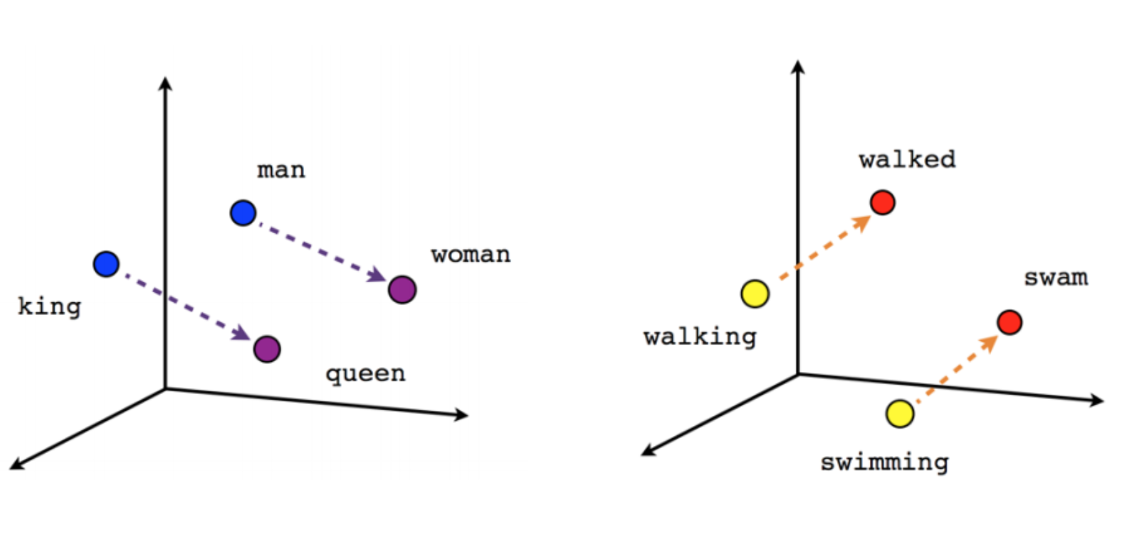
One-hot matrices, on the other hand, contain no linguistic information. (If you’re taking all the recommended detours, you’ll remember one-hot matrices from the TensorFlow MNIST digit classification tutorial.) They’re naïve; they indicate what data they contain but suggest nothing about that data, or its relationship to other information. I decided to use one-hot matrices so that I could focus on other aspects of the other project. So let’s talk about them for a bit.
Enter the (one-hot) matrix
One-hot matrices are called “one-hot” because they each embody one dimension of difference from each other; each matrix has one distinguishing (“hot”) characteristic. We can take all the data in our system and represent them using this flattened system. As an example, let’s take a couple of lines from PEP 20:
Complex is better than complicated.
Flat is better than nested.
How do we represent that in a one-hot matrix?
We begin by tokenizing the utterance; that is, breaking it into words. We end up with
['complex', 'is', 'better', 'than', 'complicated', 'flat', 'is', 'better', 'than', 'nested']
Now we can create a lookup dictionary of all the unique words. We now have:
{
  'complex': 0,
  'is': 1,
  'better': 2,
  'than': 3,
  'complicated': 4,
  'flat': 5,
  'nested': 6,
}
Count doesn’t matter; order doesn’t matter. Each token just needs a unique identifier. Now to create the matrices: each token needs to be transformed from a string into an array. Each array is of the length of the dictionary, and each value in the dictionary that’s not the value of the current token is represented by a 0. The value of the token is represented with a 1. “Complex is better than complicated” would look like:
[
  [1, 0, 0, 0, 0, 0, 0], #complex
  [0, 1, 0, 0, 0, 0, 0], #is
  [0, 0, 1, 0, 0, 0, 0], #better
  [0, 0, 0, 1, 0, 0, 0], #than
  [0, 0, 0, 0, 1, 0, 0], #complicated
]
Now we can deal with the tokens in a uniform way, since they’re all represented by isomorphic data structures, and once we’re done we can look up their values using the dictionary we made earlier.
One-hot matrices get large quickly. In my example, I’m “only” using the top 3000 most-commonly occurring words in the training corpus. This means that each word becomes represented by an array 3000 items long 😬 Whether using one-hot matrices or not, we’re reckoning with a ton of data, but one-hot matrices are ideally used for a small or finite dataset. In MNIST, for example, a one-hot matrix is used to encode information about whether an image represents a digit from 0 to 9. All the arrays are kept nice and small to a length of 10.
Let’s get cooking
Enough preamble; time to get started actually building our neural net! Our work will be based on the Reuters example in the Keras github repo, but we’ll use our own data set and make a couple more tweaks on the way.
I will be going over all the code in detail, but I have published it in full in a gist. It doesn't have a ton of backstory but it does have all the code in one nice place for you.
Neural nets can take anywhere from a few moments to days to train, depending on your hardware and on how large and/or complex your dataset is. This net took me ~60 minutes to train on a mid-2015 MacBook Pro (and it got NOISY 😅 ). My point is, you probably won’t want to have to train the net every single time you want to use it. The last step of our training script will also save the net so that we can “boot it up” quickly from another script when we actually want to consult it.
Let’s worry about the training script first. We’ll need to:
- Get our data into a usable format
- Build our neural net
- Train it with said data
- Save the neural net for future use
Organizing our data
We’re using the Twitter Sentiment Analysis Dataset available via ThinkNook. Be prepared; this dataset is extremely large and may take forever-ish to open in Excel (I had more success with Numbers).
One you open it, you can see a massive table that starts with this:
| ItemID | Sentiment | SentimentSource | SentimentText |
|---|---|---|---|
| 1 | 0 | Sentiment140 | is so sad for my APL friend............. |
| 2 | 0 | Sentiment140 | I missed the New Moon trailer... |
| 3 | 1 | Sentiment140 | omg its already 7:30 :O |
The only columns we’re interested in here are 1 and 3 — we’ll be training our net on inputs of column SentimentText with outputs of Sentiment.
We need to convert SentimentText utterances to one-hot matrices, and create a dictionary of all the words we keep track of. Here, the numpy library is your friend. I hadn’t used it much before this but it’s super powerful and has some really useful built-in utilities.
import numpy as np

# extract data from a csv
# notice the cool options to skip lines at the beginning
# and to only take data from certain columns
training = np.genfromtxt('path/to/your/data.csv', delimiter=',', skip_header=1, usecols=(1, 3), dtype=None)

# create our training data from the tweets
train_x = [x[1] for x in training]
# index all the sentiment labels
train_y = np.asarray([x[0] for x in training])
Okay, we’ve indexed all of our data; time to use Keras to make it machine-friendly.
import json
import keras
import keras.preprocessing.text as kpt
from keras.preprocessing.text import Tokenizer

# only work with the 3000 most popular words found in our dataset
max_words = 3000

# create a new Tokenizer
tokenizer = Tokenizer(num_words=max_words)
# feed our tweets to the Tokenizer
tokenizer.fit_on_texts(train_x)

# Tokenizers come with a convenient list of words and IDs
dictionary = tokenizer.word_index
# Let's save this out so we can use it later
with open('dictionary.json', 'w') as dictionary_file:
    json.dump(dictionary, dictionary_file)


def convert_text_to_index_array(text):
    # one really important thing that `text_to_word_sequence` does
    # is make all texts the same length -- in this case, the length
    # of the longest text in the set.
    return [dictionary[word] for word in kpt.text_to_word_sequence(text)]

allWordIndices = []
# for each tweet, change each token to its ID in the Tokenizer's word_index
for text in train_x:
    wordIndices = convert_text_to_index_array(text)
    allWordIndices.append(wordIndices)

# now we have a list of all tweets converted to index arrays.
# cast as an array for future usage.
allWordIndices = np.asarray(allWordIndices)

# create one-hot matrices out of the indexed tweets
train_x = tokenizer.sequences_to_matrix(allWordIndices, mode='binary')
# treat the labels as categories
train_y = keras.utils.to_categorical(train_y, 2)
✨ Cooooooooooooool. ✨ Now you have training data and labels that you’ll be able to pipe right into your neural net.
Making a model
Keras makes building neural nets as simple as possible, to the point where you can add a layer to the network in short line of code. Here’s how I built my net:
from keras.models import Sequential
from keras.layers import Dense, Dropout, Activation

model = Sequential()
model.add(Dense(512, input_shape=(max_words,), activation='relu'))
model.add(Dropout(0.5))
model.add(Dense(256, activation='sigmoid'))
model.add(Dropout(0.5))
model.add(Dense(2, activation='softmax'))
Looks simple enough. What does it mean?? 🌈🌈
Keras’ Sequential() is a simple type of neural net that consists of a “stack” of layers executed in order.
If we wanted to, we could make a stack of only two layers (input and output) to make a complete neural net — without hidden layers, it wouldn’t be considered a deep neural net.
The input and output layers are the most important, since they determine the overall shape of the neural net. You need to know what kind of input to expect, and what kind of output you want.
A representation of a neural net for identifying digits using the MNIST dataset. Source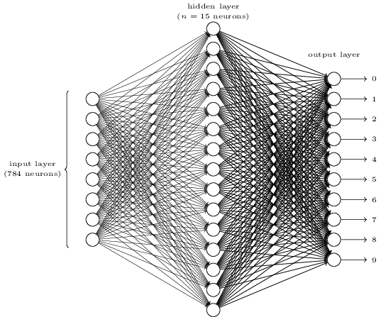
Out network will mostly consist of Dense layers — the “standard”, linear neural net layer of inputs, weights, and outputs.
In our case, we’re inputting a sentence that will be converted to a one-hot matrix of length max_words — here, 3000. We also include how many outputs we want to come out of that layer (512, for funsies) and what kind of maximization (or “activation”) function to use.
Activation functions are used when training the network; they tell the network how to judge when a weight for a particular node has created a good fit. In the first layer, I use relu (also for funsies). Activation functions differ, mostly in speed, but all the ones available in Keras and TensorFlow are viable; feel free to play around with them. If you don’t explicitly add an activation function, that layer will use a linear one.
Our output layer consists of two possible outputs, since that’s how many categories our data could get sorted into. If you use a neural net to predict rather than classify, you’re actually creating a neural net with one possible output — the prediction.
In between the input and output layers, we have one more Dense layer and two Dropout layers. Dropouts are used to randomly remove data, which can help avoid overfitting. Overfitting can happen when you keep training on the same or overly-similar data — as you train, your accuracy will hold steady or drop instead of rising.
As the last step before training, we need to compile the network:
model.compile(loss='categorical_crossentropy',
  optimizer='adam',
  metrics=['accuracy'])
Specifying that we want to collect the accuracy metric will give us really helpful live output as we train our model.
How to train your network
This is some tiny code that will take a while to run:
model.fit(train_x, train_y,
  batch_size=32,
  epochs=5,
  verbose=1,
  validation_split=0.1,
  shuffle=True)
We’re fitting (training) our model off of inputs train_x and categories train_y. We evaluate data in groups of batch_size, checking the network’s accuracy, tweaking node weights, and then running through another batch. Small batches let you train networks much more quickly than if you tried to use a batch the size of your entire training dataset.
epochs is how many times you do this batch-by-batch splitting. I’ve found 5 to be good in this case; I tried 7, but ended up overfitting.
validation_split says how much of your input you want to be reserved for testing data — essential for seeing how accurate your network is at that point. Recommended training-to-test ratios are 80:20 or 90:10. You don’t want to compromise the size of your training corpus, but you need enough test data to actually see how your net is doing.
Now go get coffee, or maybe a meal. And if you’re on a laptop, make sure it’s plugged in — training can be a real battery killer ☠️
If you need something to lose yourself in for about an hour, I suggest the Perspectiva Corporum Regularium.
As you train the neural net, Keras will output running stats on what epoch you’re in, how much time is left in that epoch of training, and current accuracy. The value to watch is not acc but val_acc, or Validation Accuracy. This is your neural net's score when predicting values for data in your validation split.
Your accuracy should start out low per epoch and rise throughout the epoch; it should increase at least a little across epochs. If your accuracy starts decreasing, you’re overfitting.
This is some sample output from training using this code over five epochs:
1420764/1420764 [==============================] - 780s - loss: 0.4947 - acc: 0.7610 - val_loss: 0.4500 - val_acc: 0.7884
Epoch 2/5
1420764/1420764 [==============================] - 850s - loss: 0.4737 - acc: 0.7760 - val_loss: 0.4481 - val_acc: 0.7902
Epoch 3/5
1420764/1420764 [==============================] - 788s - loss: 0.4662 - acc: 0.7817 - val_loss: 0.4446 - val_acc: 0.7921
Epoch 4/5
1420764/1420764 [==============================] - 819s - loss: 0.4607 - acc: 0.7859 - val_loss: 0.4471 - val_acc: 0.7921
Epoch 5/5
1420764/1420764 [==============================] - 829s - loss: 0.4569 - acc: 0.7887 - val_loss: 0.4439 - val_acc: 0.7927
Our accuracy increases from 78.8% accurate by the end of Epoch 1 to 79.3% at the end of Epoch 5.

Saving your model
Once you’re done training, it’s time to save your net so that you don’t have to keep repeating all of those steps.
Your model gets saved in two parts: One is the model’s structure itself; the other is the weights used in those model’s nodes.
model_json = model.to_json()
with open('model.json', 'w') as json_file:
    json_file.write(model_json)

model.save_weights('model.h5')
And that’s it!
Party time
Finally you can use your neural net! In a new file, you’ll open the model, its weights, and your dictionary, and then put those together to classify text. We’re going to go over the whole file at once because I’m excited to actually use it:
import json
import numpy as np
import keras
import keras.preprocessing.text as kpt
from keras.preprocessing.text import Tokenizer
from keras.models import model_from_json

# we're still going to use a Tokenizer here, but we don't need to fit it
tokenizer = Tokenizer(num_words=3000)
# for human-friendly printing
labels = ['negative', 'positive']

# read in our saved dictionary
with open('dictionary.json', 'r') as dictionary_file:
    dictionary = json.load(dictionary_file)

# this utility makes sure that all the words in your input
# are registered in the dictionary
# before trying to turn them into a matrix.
def convert_text_to_index_array(text):
    words = kpt.text_to_word_sequence(text)
    wordIndices = []
    for word in words:
        if word in dictionary:
            wordIndices.append(dictionary[word])
        else:
            print("'%s' not in training corpus; ignoring." %(word))
    return wordIndices

# read in your saved model structure
json_file = open('model.json', 'r')
loaded_model_json = json_file.read()
json_file.close()
# and create a model from that
model = model_from_json(loaded_model_json)
# and weight your nodes with your saved values
model.load_weights('model.h5')

# okay here's the interactive part
while 1:
    evalSentence = raw_input('Input a sentence to be evaluated, or Enter to quit: ')

    if len(evalSentence) == 0:
        break

    # format your input for the neural net
    testArr = convert_text_to_index_array(evalSentence)
    input = tokenizer.sequences_to_matrix([testArr], mode='binary')
    # predict which bucket your input belongs in
    pred = model.predict(input)
    # and print it for the humons
    print("%s sentiment; %f%% confidence" % (labels[np.argmax(pred)], pred[0][np.argmax(pred)] * 100))
If you run this file, you create a new model using the saved structure, and then you get a little command prompt for input to classify.
model.predict() takes what you give it, runs it through the trained neural net, and gives you a reading of how confident it is that that input belongs in each output bucket. In our case, we have two outputs, so we have two confidence estimations that range from 0 to 1; whichever one is higher is the network’s ultimate classification of that data.
Input a sentence to be evaluated, or Enter to quit: It's alive! :D
positive sentiment; 80.760884% confidence
👌🏻
You did it!
You’ve trained your first neural net that evaluates text as expressing positive or negative sentiment. And it works well(ish):
Input a sentence to be evaluated, or Enter to quit: That went better than expected
positive sentiment; 56.355631% confidence
Input a sentence to be evaluated, or Enter to quit: That did not go as expected
negative sentiment; 86.936867% confidence
Next steps

This is a really basic neural net, and there’s a lot more I’d like to investigate. Among other things:
- You can deploy machine learning models to the cloud using Google Cloud ML — what could I do if I ported my local machine to operate on Google Cloud Platform, or if I started building new models using that service?
- I chose the option of less-powerful word indexing by using one-hot matrices instead of vector embeddings. What accuracy could I get if I started using the latter?
- Classification is great but I’d really love to work on text generation, guessing at the next most-likely word in the sequence.
All of the code in this post, plus the requirements file, is up in a Github gist.
Happy coding! And thanks for following me on this journey 🌟
Coda: How well does it work? And more on data
I’m super proud of this neural net but 79% accuracy means that it’s wrong 21% of the time.
Input a sentence to be evaluated, or Enter to quit: I wish I could show you when you are lonely or in darkness the astonishing light of your own being
negative sentiment; 87.021768% confidence
Input a sentence to be evaluated, or Enter to quit: foo bar
positive sentiment; 62.751633% confidence
🤔 🤔 Those don’t look quite right.
We can always build better models, but a lot of this is Garbage In, Garbage Out. The dataset I used is incredibly large, but looking through it, there are classifications I don’t agree with, such as marking ... health class (what a joke!) as positive. Without bringing compensation algorithms into the mix, your neural net can only be as accurate as your training data.
On that note, I encourage you to examine your training data closely. What biases or prejudices might have influenced that information? Those biases will also be present, explicitly or implicitly, in your output.
The past is a very racist place. And we only have data from the past to train Artificial Intelligence. Trevor Paglen
This doesn’t mean that any and all data are inherently biased and therefore unusable — we just need to be aware of that bias and work to eradicate it. Researchers from Boston University and Microsoft have created ways to work with appropriately gendered analogies without reinforcing gender stereotypes. AI Now is an entire research organization dedicated to teasing out the biases and impacts of artificial intelligence and machine learning.
ML is powerful and we can make amazing things with it. Let’s use it to create a more equitable future.